TRANSP
MITIM can be used to run TRANSP, interpret results and plot relevant quantities. This framework does not provide licenses or support to run TRANSP, therefore, please see Installation for information on how to get TRANSP working and how to configure your setup.
Once setup has been successful, the following regression test should run smoothly:
python3 MITIM-fusion/tests/capability_tests/transp_01_run.py
Run TRANSP
For this tutorial we will need the following modules:
import os
from pathlib import Path
from mitim_tools.transp_tools import TRANSPtools
TRANSP runs are very personal and specific to each tokamak and plasma, as diagnostic availability strongly varies and namelist settings are not standarized. For this reason, this workflow assumes that a folder exists with all the plasma information (UFILES) and namelist required to run TRANSP:
folder_original = Path("MITIM-fusion/tests/data/FolderTRANSP/")
folder                  = Path("MITIM-fusion/tests/scratch/transp_tut/")
shutil.rmtree(folder)
shutil.copytree(folder_original, folder, dirs_exist_ok=True)
First, one would initialize the TRANSP class with the given folder and the tokamak name:
tokamak = "CMOD"
transp  = TRANSPtools.TRANSP( folder, tokamak )
Then, select a shotnumber and run name, such that the TRANSP simulation will have the complete name shotnumber+runname, and the MPI settings for the TRANSP run:
shotnumber  = "12345"
runname     = "X01"
mpisettings = { "trmpi": 1, "toricmpi": 64, "ptrmpi": 1 }

transp.defineRunParameters( shotnumber+runname, shotnumber, mpisettings = mpisettings )
Submit the TRANSP run:
transp.run()
Check every 5min if the run has finished, and grab final results when they are ready:
transp.checkUntilFinished( label = runname, checkMin = 5 )
Once the run has finished, results can be plotted:
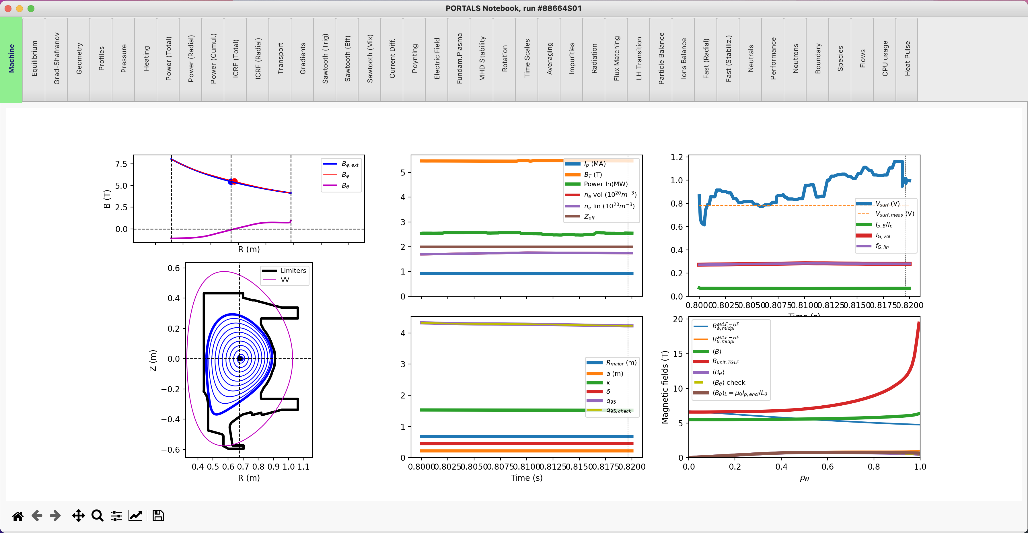
transp.plot( label = runname )
As a result, a TRANSP notebook with different tabs will be opened with all relevant output quantities:
Read results from external TRANSP run
If TRANSP has already been run and the .CDF results file already exists (cdf_file), the workflow in the previous section is not needed and one can simply read and plot the results:
from mitim_tools.transp_tools import CDFtools

transp_results = CDFtools.transp_output( cdf_file )

transp_results.plot()
Tip
transp_results is a class that parses important TRANSP outputs.
For example, to plot the electron temperature (in keV) as a function of the square root of the normalized toroidal flux coordinate at the top of the last simulated sawtooth (or last simulated time if no sawtooth present):
import matplotlib.pyplot as plt

plt.ion(); fig, ax = plt.subplots()

index_sawtooth = transp_results.ind_saw
rho            = transp_results.x[index_sawtooth,:]
TeKeV          = transp_results.Te[index_sawtooth,:]

ax.plot(rho,TeKeV)
To plot all important time and spatial variables (at time t1 seconds), simply do:
transp_results.plot( time = t1 )
Note
The contents of the TRANSP class transp_output can be found in transp_tools.CDFtools.py if one wants to understand what post-processing is applied to TRANSP outputs and the units of the variables.
TRANSP aliases
MITIM provides a few useful aliases, including for the TRANSP tools: Shell Scripts